Sound Images
Sound and Vibration
ACOUSTIC IMAGING
The terminology 2d or 3d systems for building acoustics imaging, can be misleading and it is more appropriate to present the systems as spherical or planar antennas, while the algorithms of reconstruction of acoustic fields belong to two categories: Acoustic Holography and Beamforming.
ALGORITHM – Acoustics Holography and Beamforming
The technique of Beamforming is quite similar to the principle used by a radar to identify objects in space 3d: the radar works on GHz, the Beamforming on the Hz / kHz. It is therefore to consider the Beamforming as a system capable of focusing to a source, however, instead of moving the antenna (as does the radar) to find the maximum signal, the antenna “planar” is fixed and artificial delays are introduced among the the microphones in the array that simulate virtually the focus.
The technique for Acoustic Holography assumes that the distribution 2-d of the sound pressure (amplitude and phase) on a plane (plane of measurement) satisfies the wave equation in an area external to the source (propagation) and is based on the use of algorithms of spatial transformation of acoustic fields; by simplifying the concept it can be said that a Fourier transform is applied in the spatial domain.
The acoustic holography has always been associated primarily with the analysis of the acoustic field near the source (near field) from measurements of sound pressure and / or particle velocity (intensity) carried on a plane (plane of measurement) at a certain distance from the source.
In the common bibliography the terminology established are abbreviations such NAH and SONAH, which respectively mean Near-Field Acoustic Holography and Statistically Optimized Near-Field Acoustic Holography.
ANTENNAS – Acoustic Holography
A planar antenna extent on the plane and is normally oriented towards the source, in doing so the measurement plane can be moved in the space closer to or far from the plane of the source (parallel to measurement plane). There are no particular restrictions in translating the measuring plane with the acoustic holography, the limits are defined by the antenna maximum width in regard to the minimum frequency and the minimum distance between microphones for the maximum frequency, while the spatial resolution for separation “visual source discrimination” of 2 adjacent sources is given by the distance R between the measurement plane and the source: the lower the value of R and the better the resolution.
The value of R shall not be less than the distance between the microphones, for which the order of magnitude is between 10 and 30 cm.
ANTENNAS – Beamforming
The spatial resolution Dx is in this case given by the ratio between the wavelength diameter D of the matrix (array) multiplied by the distance R between the antenna plane and source.cae-formula-bemaforming
Examples:
If R = 1 m, D = 0.8m, at 800Hz: Dx = 0.5m
If R = 1 m, D = 0.8m, to 2500Hz: Dx = 0.17m
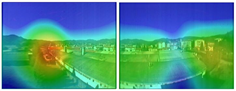
Spherical ANTENNAS – Beamforming
Spherical antenna works on the same principle of planar ones even if all the algorithms are much more complex, and there are two versions: open and closed sphere SBM (Sphere Baffled Microphone array). Considering the closed sphere is clear that the advantage over planar antenna is the fact that the sound field “can be seen” in the surrounding space (3d), while the price you have to pay is necessarily the limitation to the frequency range, whereas 1m diameter spherical antennas have very poor handling aspects.
In fact can be considered 2-3 models of antenna spherical baffled with diameters between 260 and 165 mm, whose corresponding intervals in frequency of use, it is between 200/315 Hz low frequency and 5/8 kHz in high frequency. The Noise Vision is optimized with 31 microphones and 12 cameras.